Tutorial
Table of contents
This tutorial assumes that you have a basic understanding of Python programming. If you are not familiar with Python, we recommend taking the Python for Everybody course on the Coursera platform, as shown in the following URL:
- Python for Everybody: https://www.coursera.org/specializations/python
We also recommend taking a look at the following Python course documentation:
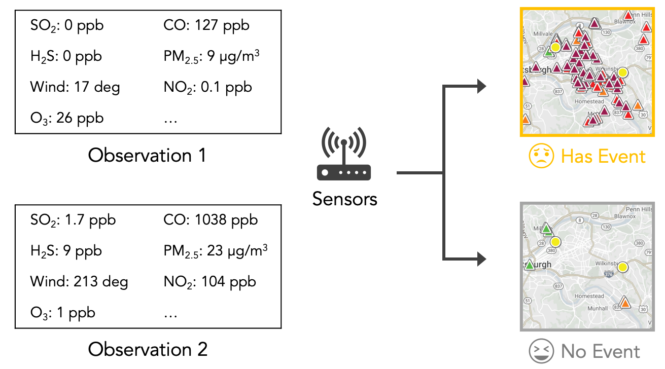
This tutorial will familiarize you with the machine learning pipeline of processing structured data, using a real-world example of building a model to predict the presence of bad smell events in Pittsburgh using air quality and weather data, as indicated in the following figure. The model is used to send push notifications about bad smell events to inform citizens. The geographical regions that we use is in Figure 6 in the Smell Pittsburgh paper.
The design brief is in the introduction section of the paper as indicated in Task 1. We will use the same dataset as used in the Smell Pittsburgh paper as an example of structured data. During the tutorial, we will explain what the variables in the dataset mean. First, go to Replit (https://replit.com/repls) and prepare to import a GitHub repository.

Next, copy the following GitHub URL and paste it into Replit’s user interface to import the code and data from the repository.
- Link to the GitHub repository: https://github.com/aml4design/smell-pittsburgh-tutorial

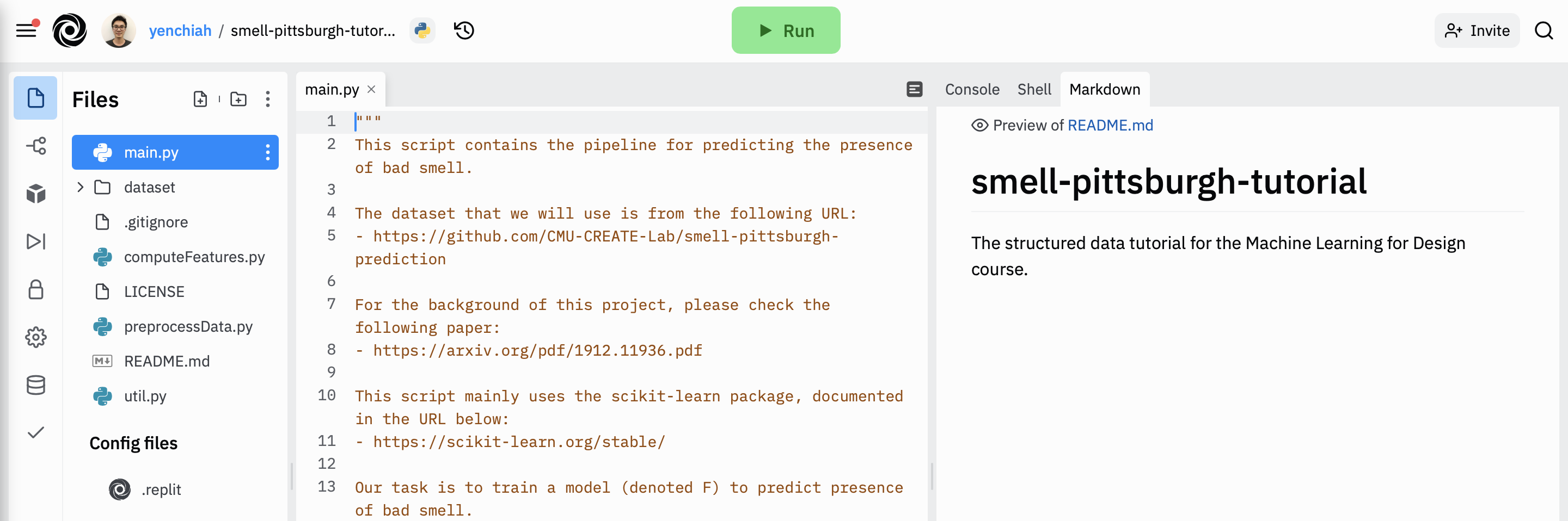
Then, wait until Replit finishes importing the repository. The folder structure and user interface in your Replit project should look like the following.
Next, click the green “Run” button at the top of the user interface to run the “main.py” script. Replit should begin installing packages automatically, which will take some time. After installing packages, the script should run without errors. In the console, you will see many messages printed by the script. The code in the script has explanations about the printed messages. The script contains a machine learning pipeline with the following steps.
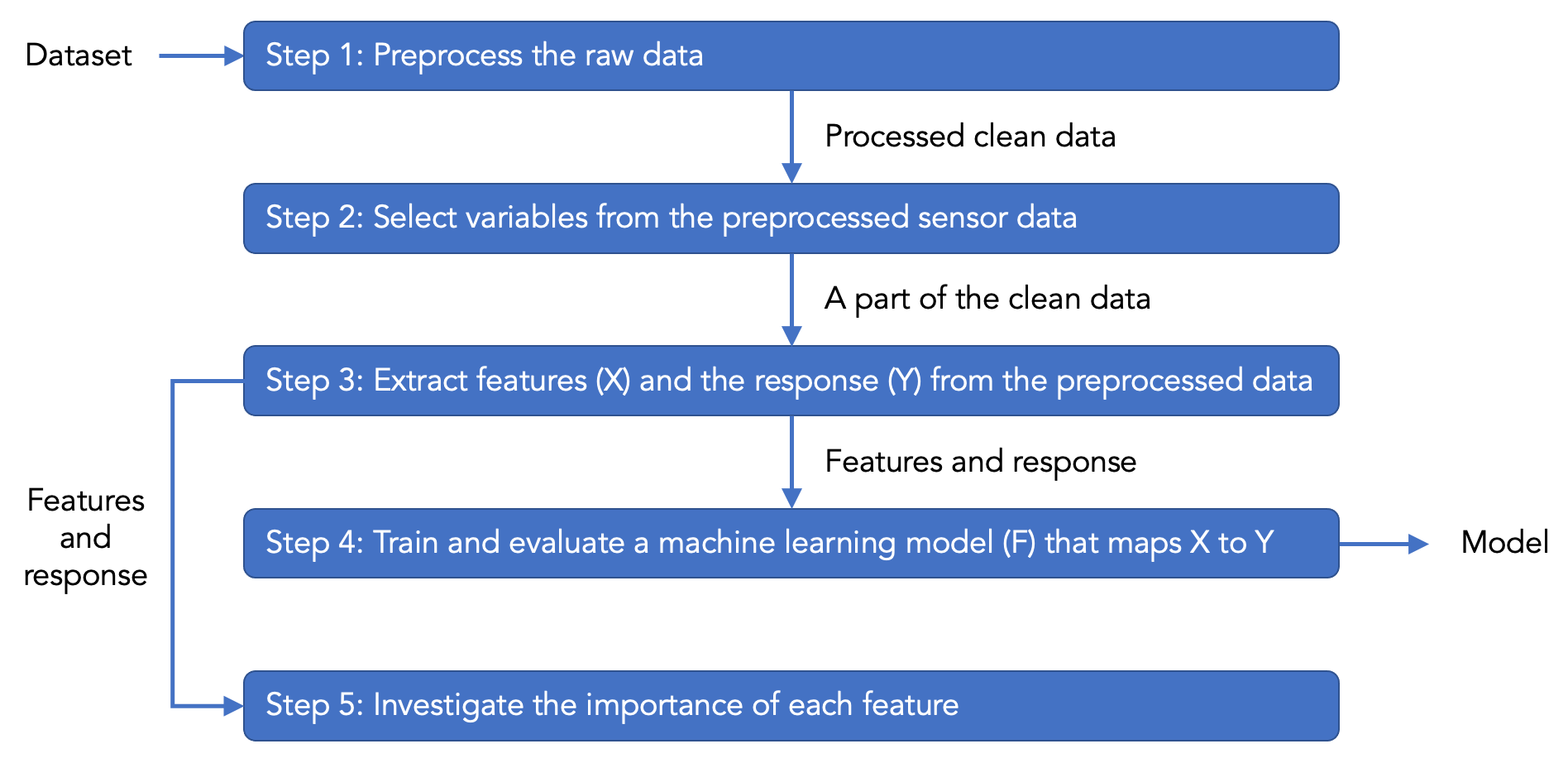
The code in the script is separated by several big blocks of comments, where each block has explanations about how the corresponding step (as shown in the above figure) works. For details about each step, please read the comments in the code.
Initially, during step 2 of selecting variables, the script uses only H2S (hydrogen sulfide) data from feed ID 28, which represents an air quality monitoring station. Every monitoring station has a unique feed ID. Some stations are operated by the municipality (which is ACHD, the Allegany County Health Department), and some of them are operated by local citizens. Every feed has several channels, for example, H2S. To find the metadata of the monitoring station, go to the following website to search using the feed ID.
- Environmental Data Website: https://environmentaldata.org/
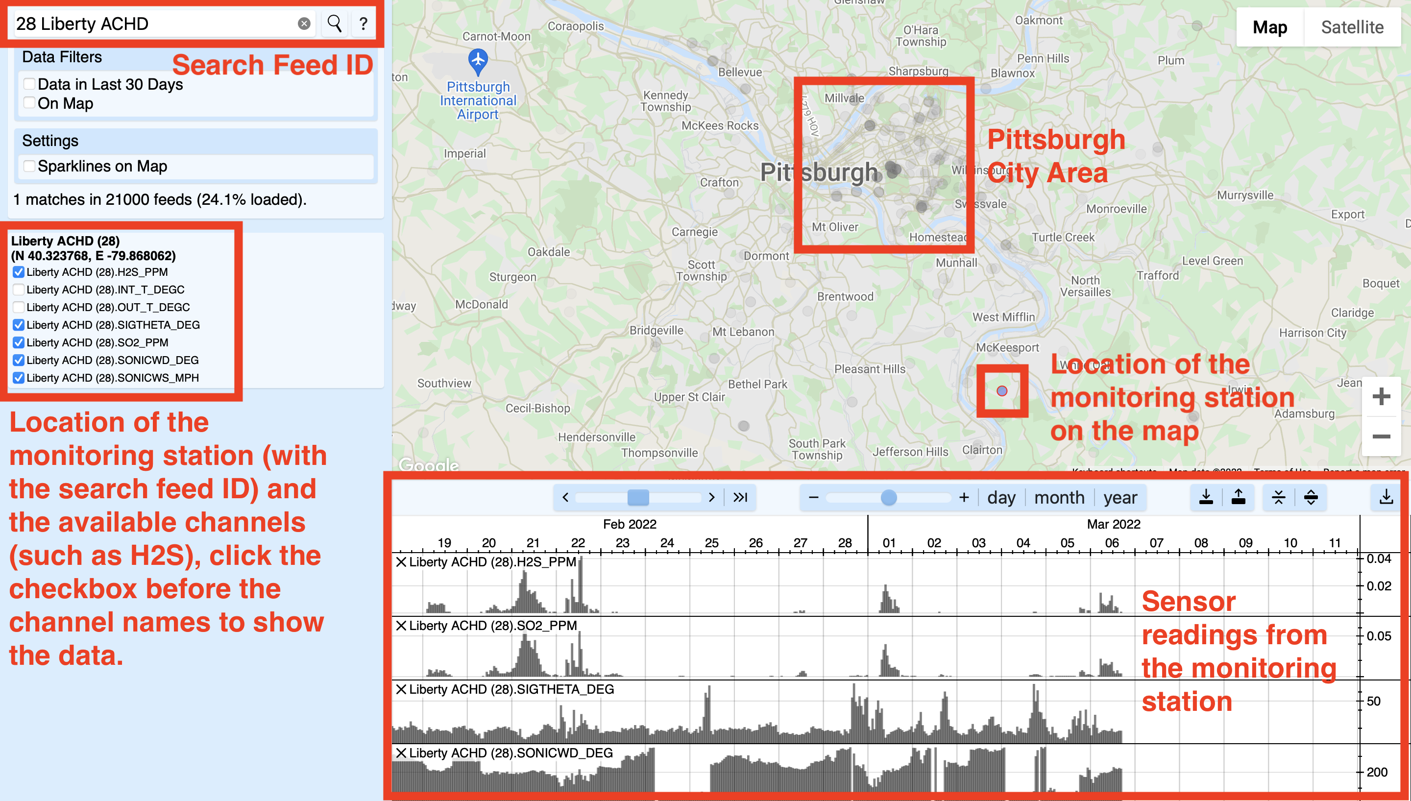
The above-mentioned website is a service that collects and visualizes environmental sensor measurements. The following screenshot shows the search result of feed ID 28, which is a monitoring station south of Pittsburgh. This monitoring station is near a major pollution source, which is the Clairton Mill Works which belongs to the United States Steel Corporation. The raw data from the monitoring station is regularly published by the ACHD.
I would encourage you to browse the data to know more about the context in Pittsburgh. The following list shows the URL with metadata for available air quality and weather variables in the dataset, which may help you do the assignments. The variable names (i.e., column names) are provided under the corresponding feed. Notice that some monitoring stations were replaced by others at some time point, so some variables in the dataset represent the combination of multiple channels or feeds, which is explained in the comments in the Python script. You will need to use the following list to decide which variables you want to use in the group assignment to inspect the effect of different features in predicting the presence of bad odors in the Pittsburgh city area.
- Feed 26: Lawrenceville ACHD
- 3.feed_26.OZONE_PPM
- 3.feed_26.PM25B_UG_M3
- 3.feed_26.PM10B_UG_M3
- 3.feed_26.SONICWS_MPH
- 3.feed_26.SONICWD_DEG
- 3.feed_26.SIGTHETA_DEG
- Feed 28: Liberty ACHD
- 3.feed_28.H2S_PPM
- 3.feed_28.SO2_PPM
- 3.feed_28.SIGTHETA_DEG
- 3.feed_28.SONICWD_DEG
- 3.feed_28.SONICWS_MPH
- Feed 23: Flag Plaza ACHD
- 3.feed_23.CO_PPM
- 3.feed_23.PM10_UG_M3
- Combination of the variables from Feed 43: Parkway East ACHD and Feed 11067: Parkway East Near Road ACHD
- 3.feed_11067.CO_PPB..3.feed_43.CO_PPB
- 3.feed_11067.NO2_PPB..3.feed_43.NO2_PPB
- 3.feed_11067.NOX_PPB..3.feed_43.NOX_PPB
- 3.feed_11067.NO_PPB..3.feed_43.NO_PPB
- 3.feed_11067.PM25T_UG_M3..3.feed_43.PM25T_UG_M3
- 3.feed_11067.SIGTHETA_DEG..3.feed_43.SIGTHETA_DEG
- 3.feed_11067.SONICWD_DEG..3.feed_43.SONICWD_DEG
- 3.feed_11067.SONICWS_MPH..3.feed_43.SONICWS_MPH
- Feed 1: Avalon ACHD
- 3.feed_1.PM25B_UG_M3..3.feed_1.PM25T_UG_M3
- 3.feed_1.SO2_PPM
- 3.feed_1.H2S_PPM
- 3.feed_1.SIGTHETA_DEG
- 3.feed_1.SONICWD_DEG
- 3.feed_1.SONICWS_MPH
- Feed 27: Lawrenceville 2 ACHD
- 3.feed_27.NO_PPB
- 3.feed_27.NOY_PPB
- 3.feed_27.CO_PPB
- 3.feed_27.SO2_PPB
- Feed 29: Liberty 2 ACHD
- 3.feed_29.PM10_UG_M3
- 3.feed_29.PM25_UG_M3
- Feed 3: North Braddock ACHD
- 3.feed_3.SO2_PPM
- 3.feed_3.SONICWD_DEG
- 3.feed_3.SONICWS_MPH
- 3.feed_3.SIGTHETA_DEG
- 3.feed_3.PM10B_UG_M3
- Feed 3506: BAPC 301 39TH STREET BLDG AirNow
- 3.feed_3506.PM2_5
- 3.feed_3506.OZONE
- Feed 5975: Parkway East AirNow
- 3.feed_5975.PM2_5
- Feed 3508: South Allegheny High School AirNow
- 3.feed_3508.PM2_5
- Feed 24: Glassport High Street ACHD
- 3.feed_24.PM10_UG_M3
Below are explanations about the suffix of the variable names in the above list:
- SO2_PPM: sulfur dioxide in ppm (parts per million)
- SO2_PPB: sulfur dioxide in ppb (parts per billion)
- H2S_PPM: hydrogen sulfide in ppm
- SIGTHETA_DEG: standard deviation of the wind direction
- SONICWD_DEG: wind direction (the direction from which it originates) in degrees
- SONICWS_MPH: wind speed in mph (miles per hour)
- CO_PPM: carbon monoxide in ppm
- CO_PPB: carbon monoxide in ppb
- PM10_UG_M3: particulate matter (PM10) in micrograms per cubic meter
- PM10B_UG_M3: same as PM10_UG_M3
- PM25_UG_M3: fine particulate matter (PM2.5) in micrograms per cubic meter
- PM25T_UG_M3: same as PM25_UG_M3
- PM2_5: same as PM25_UG_M3
- PM25B_UG_M3: same as PM25_UG_M3
- NO_PPB: nitric oxide in ppb
- NO2_PPB: nitrogen dioxide in ppb
- NOX_PPB: sum of of NO and NO2 in ppb
- NOY_PPB: sum of all oxidized atmospheric odd-nitrogen species in ppb
- OZONE_PPM: ozone (or trioxygen) in ppm
- OZONE: same as OZONE_PPM
In step 4 of training a machine learning model to identify smell events, the script initially uses a dummy classifier that always predicts “no” smell events. In other words, the dummy classifier never predicts “yes” about the presence of smell events. Later we will guide you through using more advanced machine learning models.
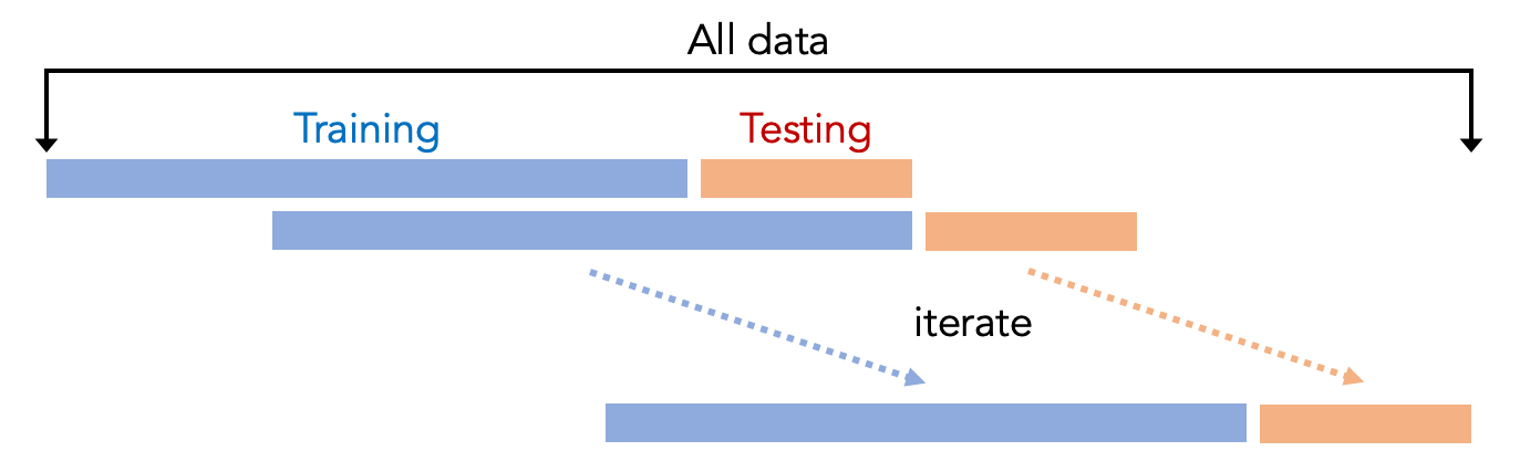
This step uses cross-validation to evaluate the machine learning model, where the data is divided into several parts, and some parts are used for training. Other parts are used for testing. Typically people use K-fold cross-validation, which means that the entire dataset is split into K parts. One part is used for testing (i.e., the testing set), and the other parts are used for training (i.e., the training set). This procedure is repeated K times so that every fold has the chance of being tested. The result is averaged to indicate the performance of the model, for example, averaged accuracy. We can then compare the results for different machine learning pipelines.
However, the script uses a different cross-validation approach, where we only use the previous folds to train the model to test future folds. For example, if we want to test the third fold, we will only use a part of the data from the first and second fold to train the model. The reason is that the Smell Pittsburgh dataset is primarily time-series data, which means the dataset has timestamps for every data record. In other words, things that happened in the past may affect the future. So, in fact, it does not make sense to use the data in the future to train a model to predict what happened in the past. Our time-series cross-validation approach is shown in the following figure.
In this script, we print the following evaluation metrics: averaged f1-score, averaged precision, averaged recall, and averaged accuracy across all the folds. These metrics are always in the range of zero and one, with zero being the worst and one being the best. We also printed the confusion matrix that contains true positives, false positives, true negatives, and false negatives. To understand the evaluation metrics, let us first take a look at the confusion matrix, explained below:
- True positives
- There is a smell event in the real world, and the model correctly predicts that there is a smell event.
- False positives
- There is no smell event in the real world, but the model falsely predicts that there is a smell event.
- True negatives
- There is no smell event in the real world, and the model correctly predicts that there is no smell event.
- False negatives
- There is a smell event in the real world, but the model falsely predicts that there is no smell event.
The accuracy metric is defined in the equation below:
accuracy = (true positives +true negatives) / total number of data points
Accuracy is the number of correct predictions divided by the total number of data points. It is a good metric if the data distribution is not skewed (i.e., the number of data records that have a bad smell and do not have a bad smell is roughly equal). But if the data is skewed, which is the case in our dataset, we will need another set of evaluation metrics: f1-score, precision, and recall. We will use an example later to explain why accuracy is an unfair metric for our dataset. The precision metric is defined in the equation below:
precision = true positives / (true positives + false positives)
In other words, precision means how precise the prediction is. High precision means that if the model predicts “yes” for smell events, it is highly likely that the prediction is correct. We want high precision because we want the model to be as precise as possible when it says there will be smell events. Next, the recall metric is defined in the equation below:
recall = true positives / (true positives + false negatives)
In other words, recall means the ability of the model to catch events. High recall means that the model has a low chance to miss the events that happen in the real world. We want high recall because we want the model to catch all smell events without missing them.
Typically, there is a tradeoff between precision and recall, and one may need to choose to go for a high precision but low recall model, or we go for a high recall but low precision model. The tradeoff depends on the context. For example, in medical applications, one may not want to miss the events (e.g., cancer) since the events are connected to patients’ quality of life. In our application of predicting smell events, we may not want the model to make false predictions when saying “yes” to smell events. The reason is that people may lose trust in the prediction model when we make real-world interventions incorrectly, such as sending push notifications to inform the users about the bad smell events.
The f1-score metric is a combination of recall and precision, as indicated below:
f1-score = 2 * (precision * recall) / (precision + recall)
In the console after you run the python script on the Replit tool, there is a message printed by the script, as shown in the following:
Use model DummyClassifier(constant=0, strategy='constant')
Perform cross-validation, please wait...

================================================
average f1-score: 0.0
average precision: 0.0
average recall: 0.0
average accuracy: 0.92
number of true positives: 0
number of false positives: 0
number of true negatives: 14914
number of false negatives: 1382
================================================
This shows the result of the model, which is the dummy classifier that always predicts “no” for the smell events. In the printed message, we see that the accuracy is 0.92, which is very high. But the f1-score, precision, and recall are zero since there are no true positives. This is because the Smell Pittsburgh dataset has a skewed distribution of smell events, which means that there are a lot of “no” (14914 data records) but only a small part of “yes” (1382 data records). This skewed data distribution corresponds to what happened in Pittsburgh. Most of the time, the odors in the city area are OK and not too bad. Occasionally, there can be very bad pollution odors, where many people complain.
By the definition of accuracy, the dummy classifier (which always says “no”) has a very high accuracy of 0.92. This is because only 8% of the data indicate bad smell events. So, you can see that accuracy is not a fair evaluation metric for the Smell Pittsburgh dataset. And instead, we need to go for the f1-score, precision, and recall metrics.
Task 4
In this task, we are going to use a different model. Now, let us change the model to Decision Tree and compare its performance with the dummy classifier. We will explain what a Decision Tree is later in this tutorial. First, please find the following line in the code:
model = DummyClassifier(strategy="constant", constant=0)
Replace the line above with the following code:
model = DecisionTreeClassifier()
Next, please find the line that imports the package in the step of training the model:
from sklearn.dummy import DummyClassifier
Replace the line above with the following code:
from sklearn.tree import DecisionTreeClassifier
Then, run the code again, and the console should print the following message:
Use model DecisionTreeClassifier()
Perform cross-validation, please wait...

================================================
average f1-score: 0.13
average precision: 0.19
average recall: 0.16
average accuracy: 0.86
number of true positives: 325
number of false positives: 1295
number of true negatives: 13619
number of false negatives: 1057
================================================
Notice that the Decision Tree model produces non-zero true positives and false positives (compared to the dummy classifier). Also, notice that f1-score, precision, and recall are no longer zero. If you did not find the message that prints the evaluation metrics, try scrolling the console printed messages and find the part that is similar to the above.
Decision Tree is a type of machine learning model. You can think of it as how a medical doctor diagnoses patients. For example, to determine if the patients need treatments, the medical doctor may ask the patients to describe symptoms. Depending on the symptoms, the doctor decides which treatment should be applied for the patient.
One can think of the smell prediction model as an air quality expert who is diagnosing the pollution patterns based on air quality and weather data. The treatment is to send a push notification to citizens to inform them of the presence of bad smell to help people plan daily activities. This decision-making process can be seen as a tree structure as shown in the following figure, where the first node is the most important factor to decide the treatment.
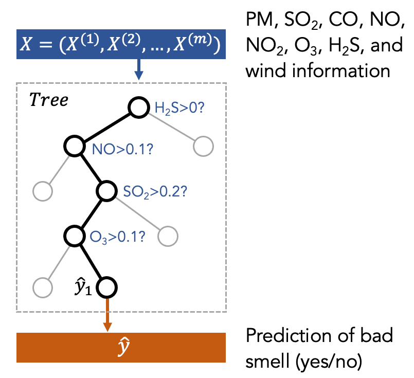
The above figure is just a toy example to show what a decision tree is. In our case, we put the features (X) into the decision tree to train it. Then, the tree will decide which feature to use and what is the threshold to split the data based on the features. This procedure is repeated several times (represented by the depth of the tree). Finally, the model will make a prediction (y) at the final node of the tree.
You can find the visualization of a decision tree (trained using the real data) in Figure 8 in the Smell Pittsburgh paper. If you have not read the paper (or want to find the link to the paper), please go back to Task 1 in this module. More information about the Decision Tree can be found in the following URL and paper:
- Decision Tree model: https://scikit-learn.org/stable/modules/tree.html
- Quinlan, J. R. (1986). Induction of decision trees. Machine learning, 1(1), 81-106.
Task 5
Now that you have tried the Decision Tree model, in this task, we will use a more advanced model for smell event prediction. The mode that we will use is Random Forest. First, similar to the first few steps in the previous task, add a line to define the Random Forest model. You can add the line right after the line where you create the Decision Tree model in the previous task. You can comment out the line that creates the Decision Tree model.
#model = DecisionTreeClassifier()
model = RandomForestClassifier()
Also, add the following line to import the package. You can add the line right after the line where you import the Decision Tree model in the previous task.
from sklearn.ensemble import RandomForestClassifier
Now, run the code again. The cross-validation part may be slow since training the Random Forest model can take a long time. After that, you should see the following message about evaluation metrics in the console:
Use model RandomForestClassifier()
Perform cross-validation, please wait...

================================================
average f1-score: 0.11
average precision: 0.19
average recall: 0.1
average accuracy: 0.9
number of true positives: 212
number of false positives: 529
number of true negatives: 14385
number of false negatives: 1170
================================================
Notice that the performance of the model does not look much better than the Decision Tree model. And in fact, both models currently have poor performance. This can have several meanings, as indicated in the following list. You will explore these questions more in the individual and group assignments.
- Firstly, do we really believe that we are using a good set of features? Is it sufficient to only use the H2S (hydrogen sulfide) variable? Is it sufficient to only include the data from the current time and the previous hour?
- Secondly, the machine learning pipeline uses 14 days of data in the past to predict smell events in the future 7 days. Do we believe that 14 days are sufficient for training a good model?
- Finally, the threshold that we used to define a bad smell event is 40, which is the sum of smell ratings that people reported within the time range that we want to predict (in our case, it is 8 hours). Do we believe that 40 is a good number to determine the presence of a bad smell?
Now let us take a look at the Random Forest model, which is a type of ensemble model. You can think about the ensemble model as a committee that makes decisions collaboratively, such as using majority voting. For example, to determine the treatment of a patient, we can ask the committee of medical doctors for a collaborative decision. The committee has several members who correspond to various machine learning models. The Random Forest model is a committee that is formed with many decision trees. Each tree is trained using different sets of data, as shown in the following figure.
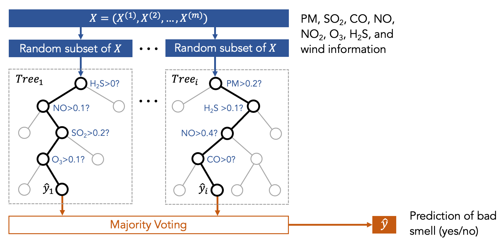
In other words, we first trained many decision trees, and each of them has access to only a part of the data (but not all of the data) that are randomly selected. So, each decision tree sees different sets of features. Then, we ask the committee members (i.e., the decision trees) to make predictions, and the final result is the one that receives the highest votes.
The intuition for having a committee (instead of only a single tree) is that we believe a diverse set of models can make better decisions collaboratively. There is mathematical proof about this intuition, but the proof is outside the scope of this course. More information about the Random Forest model can be found in the following URL and paper:
- Random Forest model: https://scikit-learn.org/stable/modules/ensemble.html
- Breiman, L. (2001). Random forests. Machine learning, 45(1), 5-32.
Also, notice that there is a message printed in the console similar to the following:
Computer feature importance using RandomForestClassifier(random_state=0)

================================================
Display feature importance based on f1-score

   feature_importance          feature_name
0             0.63188     3.feed_28.H2S_PPM
1             0.59183             HourOfDay
2             0.52891                   Day
3             0.50336  3.feed_28.H2S_PPM_1h
4             0.47280             DayOfWeek

Column names below:
['feature_importance', 'feature_name']
================================================
This part prints feature importance, which indicates the influence of each feature on the model prediction result. Here we use the Random Forest model. For example, in the printed message, the “H2S” feature has the highest importance, followed by the “hour of day” feature. The values in the feature importance here represent the decrease of f1-score if we randomly permute the data related to the feature. For example, if we randomly permute the H2S measurement for all the data records (but keep other features the same), the f1-score of the Random Forest model will drop 0.63. The intuition is that if a feature is more important, the model performance will decrease more when the feature is randomly permuted (i.e., when the data that is associated with the feature are messed up). More information can be found in the following URL:
- Link to the explanation of feature importance: https://scikit-learn.org/stable/modules/permutation_importance.html
Notice that depending on the number of features you are using, the step of computing the feature importance can take a lot of time.